Now that we have a solid understanding of the basic concepts of statistics, we can finally tie them together with the topics in quantitative science we talked about in Psychology as a Science last term, and learn how we can use statistics to find out about the world.

We’ll start by refreshing our memory about scientific hypotheses and talk about how we get from a research question to a conceptual, operational, and finally statistical hypothesis. After that we’ll learn how we can statistically test hypotheses in a framework called Null Hypothesis Significance Testing. In doing so, we’ll introduce a crucial concept of this framework, the p-value.

Hypothesis

Let’s start by going over what we already know about quantitative scientific methodology.

The purpose of quantitative science is to derive generalisable knowledge based on observation. This knowledge is systematised in the form of scientific theories: frameworks that describe, explain, and predict some aspect of the universe. Theories have the ability to generate hypotheses which are simply testable statements about the world. These statements are often framed in terms of differences or relationships between things, people, or groups.

In order for a statement to qualify as a scientific hypothesis, it must be empirically testable. That means that it must be possible, at least in principle, to find empirical observations (data) that support or disconfirm the hypothesis. In other words, it must be clear what data we’re expecting to see if the hypothesis is correct and what data we could observe that would prove the hypothesis false.

There are several ways in which we can formulate a hypothesis, each with its own place in the scientific process.

Levels of hypotheses

Conceptual level

Research often starts with a question about something in the world that piqued the interest of the researcher. The first step towards quantitative research is to come up with a conceptual hypothesis that formulates the main part of the research question as a single testable statement about one particular effect or relationship. Conceptual hypotheses are expressed in normal language and, as the name suggests, deal with concepts or constructs.

To illustrate, take this example of a good conceptual hypothesis:

“The recent observed rising trend in global temperatures on Earth is primarily driven by human-produced greenhouse gas emissions.”

The hypothesis posits a clear relationship between human-produced greenhouse gasses and global warming. It does so in a way that renders the hypothesis testable: there’s a clearly implied set of observations that would falsify this claim. For instance, if we gathered data that reliably shows that it is, for instance, solar activity that is mostly responsible for the trend, the hypothesis would be proven wrong.

It’s important to appreciate that whether or not a hypothesis is good has nothing to do with whether or not it is true. This one happens to be true¹ but we only found that out after the topic was scientifically investigated. In fact, there’s not point testing hypotheses that we know are true. The point of research is to find out new things about the world – things we do not yet know.

Contrast the above good hypothesis with a not-so-good one:

“Homœopathic products can cure people, but sometimes they make them worse before they make them better, and the effect is only apparent subjectively with respect to some vague ‘holistic’ notions rather than a specific well-defined and testable set of criteria.”

Again, whether the hypothesis is good or bad doesn’t hinge upon whether or not homœopathy works (it doesn’t) but whether or not the statement opens itself to empirical scrutiny. In this case, you’d struggle to imagine a set of observations that could, at least in principle, falsify this vague, ill-defined claim.

Operational level

Once we have arrived at a good conceptual hypothesis, it’s important to operationalise it. As you learnt last term, operationalisation is the process of defining variables in terms of how they are measured. For example, the concept of intelligence can be operationalised as total score on Raven’s Progressive Matrices or the concept of cognitive inhibition can be operationalised as (some measure of) performance on the Stroop test.

Operationalising a hypothesis allows us to think about it in terms of quantitative methodology and, ultimately, statistics.

Statistical level

The final step in hypothesis-generation involves translating the operational hypothesis to the language of mathematics/statistics. A statistical hypothesis deals with specific values (or ranges of values) of population parameters. For instance, we could hypothesise that the mean of a given population has a certain value or that there is a difference in means between two populations.

Restating a hypothesis in these terms allows us to test its claim using statistical tools. The remainder of this lecture will walk you through the various stages of this process.

From research question to statistical hypothesis

Before we talk about how hypotheses can be statistically tested, let’s go over an example of generating a hypothesis on all three levels. Let’s say that we are interested in factors predicting sport climbing performance. What makes some people good at climbing? Maybe we are interested in investigating if there might be morphological characteristics that predispose some people to be better at climbing. This is our research question.

Let’s say that we have a hunch that having relatively long arms might be beneficial for climbing as it allows you to reach further, thus giving you a larger selection of things to hold onto. From this hunch we can formulate a conceptual hypothesis: “Climbers have relatively longer arms than non-climbers.”

In order to operationalise our hypothesis, we need a measure of this relative arm length.

The Ape Index

The ape index (AI) is a measure that compares a person’s arm span to their height. Having a positive AI means, that your arm span is larger than your height.

For instance, someone who is 165 cm (5′5″) tall and has an arm span of 167 cm, has an ape index of +2 cm (see picture below).

AI has actually been found to correlate with performance in some sports, such as climbing, swimming, or basketball.

If we choose the ape index as our measure of relative arm length, we can formulate an operational hypothesis: “Elite climbers have, on average, a higher ape index than general population.”

Notice how this reformulation defines both what we mean by “longer arms” but also the groups we are comparing. In fact, we are saying that, when it comes to arm length, elite climbers and “normal people” are two distinct populations.

Finally, translating this statement into the language of parameters gives us our statistical hypothesis: \(\mu_{\text{AI}\_climb} > \mu_{\text{AI}\_gen}\)

This inequality simply says, that the population mean of AI in (elite) climbers is higher than that of AI in the general population.

Testing hypotheses

Now that we’ve arrived at a testable statistical hypothesis, we can go out and submit the hypothesis to an empirical test.

Imagine we go to El Capitan in the Yosemite park, find a climber and measure their AI. Then we grab the first non-climber in the vicinity and measure their AI. We find that the climber has a higher AI than the non-climber. That’s it! hypothesis confirmed; we happy!

Or are we happy?

Not so fast! Obviously, we cannot conclude that our hypothesis has been confirmed because the individuals might not be representative of the populations. Sure, we can – and absolutely should – collect a larger sample than one per group but the fundamental problem remains: sample statistics (e.g., the mean) might not capture the population parameter (e.g., \(\mu\)) accurately! Having a large sample definitely helps though…

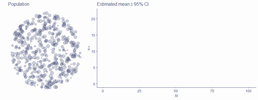
Let’s illustrate this problem with sampling using a simulation. The circle of points below represents a single population. This population has a mean of 10.

Let’s see how the population estimate \(\hat{\mu}\) behaves as a function of sample size N. (Remember that \(\hat{\mu}\) is equal to sample mean \(\bar{x}\).)

Click/tap on the picture to sample two points and imagine, that the yellow one is out climber and the brown one is our member of the general population.

Now, because both of these “groups” (a group of one person can still be a group) are sampled from the same population so they should have the same means. However, as luck would have it, we managed to sample a particularly small observation in the yellow group and a particularly large one in the brown group, yielding very different sample means.

Click on the picture again to run an animation. In this simulation, we’ll keep adding observations to each of the two groups. We’ll also add 95% confidence intervals around each estimate of the mean (the blue-grey ribbon).

Watch carefully what happens with the means as N gets larger…

Given this inherent uncertainty around parameter estimates, the question to asi is: How do we decide that a difference/effect in our sample actually exists in population?

There are various approaches to tackling this problem. The one we will focus on in this module as well as the two next research methods modules is the framework of Null Hypothesis Significance Testing (NHST). Before we delve into it, there are a few things you ought to know about it. Firstly, there is, and always has been, strong criticism of this approach. If you are interested, check out this blog post for a non-technical summary of the main sources of criticism of NHST.

Despite this criticism, the approach is very widely used in psychology and other social and biological sciences and so you need to understand it. The vast majority of research papers report statistical tests within this framework and so we’d be doing you a major disservice if we omitted NHST from your education.

Secondly, there exist alternatives to NHST. One that has gathered a lot of traction in the past 20 years is so-called Bayesian inference. We will, however, not be introducing this topic in your undergrad modules.

With that our of the way, let’s talk about what the Null Hypothesis Significance Testing framework actually entails.

Basically, NHST is a method of conjuring up two parallel universes and then deciding which one we live in. Sadly, is a little less exciting than it sounds but it’s still very important!

OK, there’s quite a lot to unpack here so let’s take it one step at a time

Formulate a research hypothesis

We already know how to generate a good conceptual, operational, and statistical hypothesis. Actually, let’s use the one we came up with; the one about the ape index in elite climbers Vs non-climbers. The statistical hypothesis we settled one was: \[\mu_{\text{AI}\_climb} > \mu_{\text{AI}\_gen}\] There is a directionality to this hypothesis: we claim that AI in climbers is greater than that in non-climbers. This is known as a one-tailed hypothesis for reasons that will become clear later.

In practice, however, we tend to work with two-tailed hypotheses, that is hypotheses that don’t assume a direction. The exception to this convention are cases where it makes no sense to expect an effect in one of the directions but those cases are rare in psychology.

So, rather than a directional hypothesis (climbers have longer arms than non-climbers), let’s restate our hypothesis as that of some difference or effect, i.e. a two-tailed hypothesis: \[\mu_{\text{AI}\_climb} \ne \mu_{\text{AI}\_gen}\]

Formulate a null hypothesis

In the NHST framework, we actually do no test the research hypothesis. Instead, we formulate a so-called null hypothesis and submit that one to statistical testing.

The null hypothesis (or the null, for short) is simply a negation of the statistical hypothesis. In practice, it often ends up being a hypothesis about no difference or effect but this is not a requirement.

So, if our research – or alternative hypothesis – is \[H_1:\mu_{\text{AI}\_climb} \ne \mu_{\text{AI}\_gen}\] its negation – the null hypothesis – will be \[H_0:\mu_{\text{AI}\_climb} = \mu_{\text{AI}\_gen}\]

To put it in normal language, the null states that the means of AI are the same for both climbers and non-climbers: the ape indices of these two groups of people come from the same population.

It’s useful to think of these two competing hypotheses (\(H_0\) and \(H_1\)) as representing alternative realities or parallel universes. In the world of \(H_0\), there is no difference between AI in climbers and non-climbers, while in the world of \(H_1\), there is at least some difference.

Test statistic

Now that we have our hypotheses figured out, we need some kind of a measure by which we can judge whether or not our assumption that the null hypothesis is true is a reasonable one. We need some kind of a test statistic: a mathematical expression of what we’re measuring, whether that thing is some kind of a difference, effect, or relationship.

Statisticians have developed many different test statistics, each useful for a different scenario, and we’ll spend the remainder of this module learning about some of them. But for now, let’s just take simple difference in means as our sample statistic. Because it’s a difference, let’s call it D and define it as \[D = \overline{\text{AI}}_{climb}-\overline{\text{AI}}_{gen}\] where \(\overline{\text{AI}}\) is the mean ape index in the sample.

D is then a sample measure and should be reflective of the associated population difference. To keep up the convention of using Latin/Roman letters for sample statistics and Greek for population parameters, let’s call the population difference Δ (Greek capital letter delta).

Remember that in the NHST framework, we assume that the null hypothesis is true. In other words, we assume that we live in the reality, where there is no difference and so we assume that Δ = 0. If this assumption is correct, we would expect D to also be 0, because D is our best guess about Δ: \(D = \hat{\Delta}\).

Even though our best guess about the value of D that we expect to find in any sample is zero, we know that, because of statistical fluctuations inherent in sampling, we may very well observe a non-zero value of D, even though it’s sampled from a population where true Δ is indeed 0.

But in order to be more precise about these expectations, we need to know what the sampling distribution of our test statistic looks like.

Sampling distribution of the test statistic

As we explained above, the two competing hypotheses represent to alternative realities, one with a difference, one with no difference. It’s very important to understand that these two realities produce different kinds of data, which is why we have different expectations about what sorts of results we can observe if we live in the reality of the null or the reality of the alternative hypothesis.

If H₁ is true

We said that our alternative hypothesis \(H_1\) represents the world where there is a difference in average ape index between elite climbers and the general population. If this is the world we live in (if \(H_1\) is true), the true value of Δ is not zero. Sure, we could still sometimes sample data and find D very close to zero but, of average, we’d expect to find non-zero D in our data.

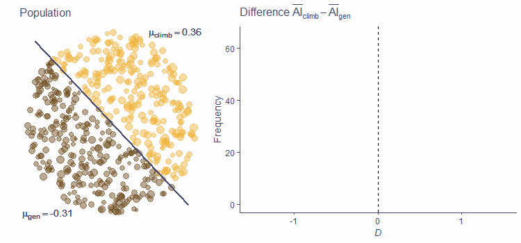
Let’s use simulation to visualise the sampling distribution of D under \(H_1\)². The circle in the picture below represents the world of \(H_1\). This world is split into two populations, elite climbers (yellow) and general population (brown). In this world, the ape indices of these two groups come from different populations, because the true Δ is not zero. In our example, the population mean AI in climbers is 0.36, while in the general population, it is −0.31. This is illustrated by the yellow circles being larger on average, but there’s also a substantial overlap in the sizes.

When you click/tap on the picture, the simulation will sample 30 points from each of the two populations, calculate D and plot its value on the histogram in the right-hand-side of the picture. Do it now!

We know that the centre of the sampling distribution of a statistic is equal to the true value of the corresponding population parameter and so we know that this histogram should be centred around 0.67. If this does not ring true yet, you absolutely must revisit the previous lectures! Click on the picture again to run an animation that will repeatedly sample from these populations, calculate D and add its value to the histogram to gradually build up a simulated sampling distribution.

As you can see, the simulated sampling distribution is indeed centred around the true value of Δ and, in the universe of \(H_1\) this value is not zero. However, notice that a few of D statistics were very close to 0, in fact, one was just on the “wrong” side of zero. These were the instances of Type II error or false negative: We found no (or next-to-no) difference even if there is one in the population.

If H₀ is true

Let us now see what the sampling distribution looks like in the alternative reality. To reiterate, \(H_0\) represents the world where there is no difference in average ape index between elite climbers and the general population. So this time, we’re sampling from the same population in the simulation below. This is depicted by there only being a single cluster of circles.

Let’s assume that \(\text{AI}_{gen}\) is normally distributed in population with \(\mu = 0\) and \(\sigma=1.53\)

If you click/tap on the picture, the simulation will randomly sample two groups of 30 from this single population and again, calculate the D and plot it on the histogram next to the cluster. This time round, we know that Δ = 0 and so the histogram too will be centred around 0. Click/tap on the picture again to run the simulation and watch the sampling distribution of D form.

Notice here that, even though the true difference in population is zero, D can be non-zero in sample. In fact, the vast majority of Ds are non-zero but, because the sampling distribution is centred around 0, the best guess remains D = 0. Also notice, that while small departures from the true value of Δ are common, large ones are relatively rare. That’s because of the bell-like (approximately normal, in fact) shape of the sampling distribution.

Because we are testing the null hypothesis, this sampling distribution centred around 0 is the one we will be using for our test. Knowing the characteristics of the sampling distribution (its mean and SD in this case) allows us to calculate the probability of observing any result we could possibly observe.

Gather data and calculate the test statistic

Now that we know what our test statistic is and how it is distributed in the world of \(H_0\), we can go out and collect data. There isn’t much we can say about this step in the process here but it is the main part of any study. Collecting data requires careful design, planning, and execution but these methodological concerns are not within the scope of this lecture.

So let’s just imagine we went out and measure the ape index of 30 elite climbers and 30 members of the general population. We calculated the mean difference D and found that, in our sample, it was 0.47. In other words, climbers had, on average larger AI than non-climbers by 0.47 cm.

Calculate probability of observed statistic under H₀

Because we know what the sampling distribution od D under the null hypothesis looks like, we can calculate the probability of finding a D of 0.47 or larger if we actually sampled the date in the world of \(H_0\). Remember, we don’t know which of the two parallel universes we inhabit and so we assume it’s the \(H_0\) one and look if the data we observe are consistent with this assumption.

Here is the sampling distribution from the simulation above. It’s not the actual sampling distribution because we only sampled about 1,000 samples and no an infinity of them. Click/tap on the picture to see the ideal shape of the sampling distribution.

Because we know the parameters of this distribution, we can calculate the probability of sampling an arbitrary range of values from this distribution. This probability is simply the area below the curve between two arbitrary cut-off points. Click on the picture again to see a few of such points.

Because we can calculate the area between any set of points, we can see what proportion of this distribution is larger or equal to our value of D.

OK, one more click/tap to see if you were right (within rounding error).

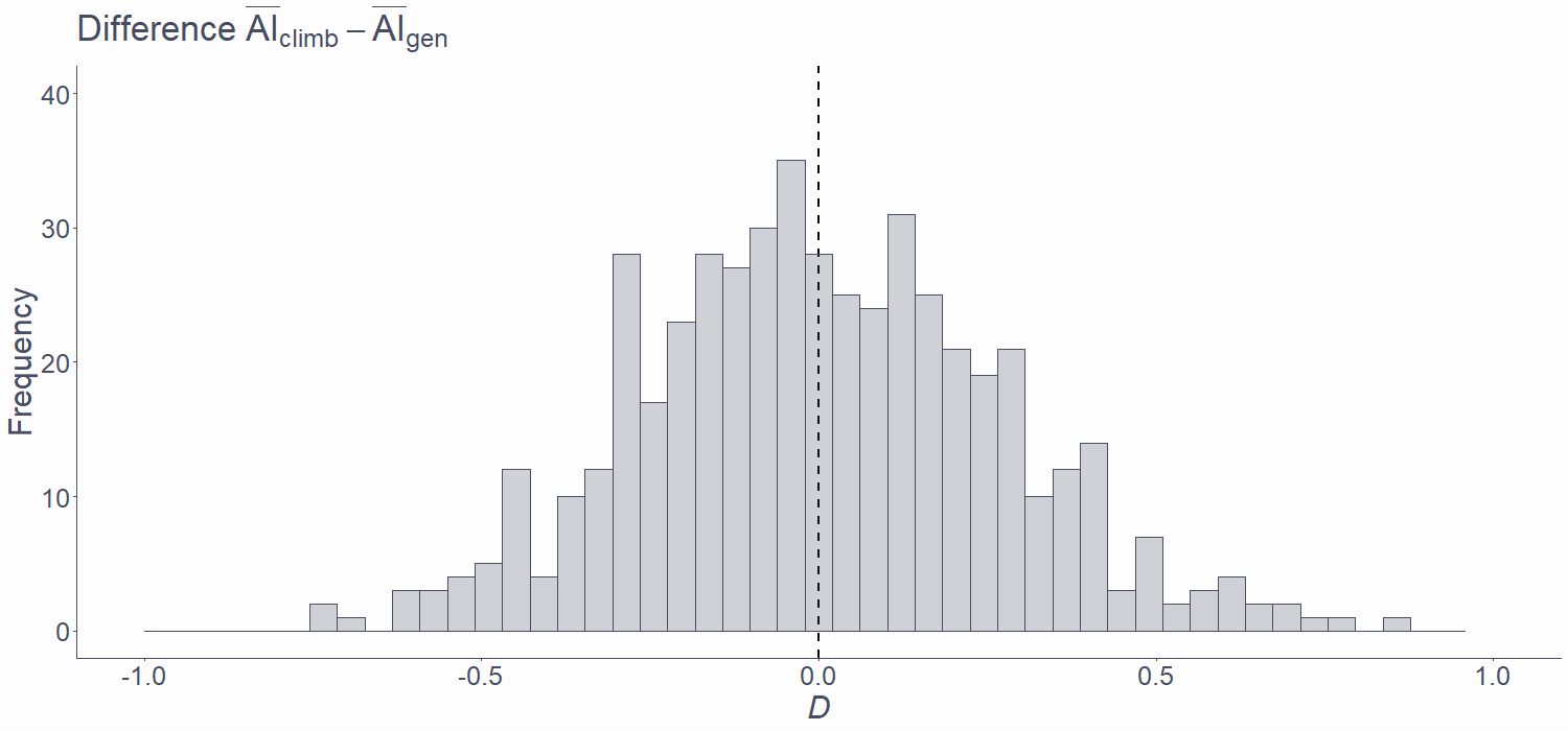
So, by comparing the value of D that we observed in our sample to the sampling distribution of this test statistic, we found that the probability of getting a D ≥ 0.47 is .047. However, because our \(H_0\) states that Δ = 0, we need to consider the opposite tail of the distribution as well. In other words, we want the 2-tailed probability: the combined probability that D is greater than or equal to 0.47 or that it is smaller than or equal to −0.47. The joint probability of these two events is just twice the original probability: .094. This is because the sampling distribution is centred around 0 and symmetrical and so the area under the left-hand tail up until −0.47 is equal to that under the right-hand tail from 0.47 on.

This probability is called the p-value in the NHST framework and it is an extremely important concept to understand correctly.

Decision

Now that we know how likely our data are under \(H_0\), it’s time to decide whether we think we live in the universe of \(H_0\) or \(H_1\).

To summarise our progress thus far, we have:

• Data
• Test statistic D
• Distribution of test statistic under \(H_0\)
• Probability of our test statistic or a more extreme one under \(H_0\) (p-value)

So how do we reach our decision about which of the two worlds we live in?

Well, we reject \(H_0\) (the assumption that we live in the world of no difference) and accept \(H_1\) if we judge our result to be sufficiently unlikely in the world of \(H_0\). Conversely, we retain \(H_0\) if we judge the result to be likely under it because, in that case, our data are not inconsistent enough with the assumption that there is no difference.

That’s all very well but exactly how unlikely is unlikely enough?

The answer to this question is always a matter of arbitrary choice! There is no single p-value woven into the fabric of the universe that tells us whether we should accept our research hypothesis or retain the null.

That said, there are a few commonly used cut-off for retaining or rejecting the null. Before we even collect our data, we should choose a so-called significance level also known as \(\alpha\) level that we will use as criterion for deciding which of the two realities we inhabit.

Again, the particular significance level is arbitrary but the most commonly chosen ones are:

• 5%, or .05 (most common),
• 1%, or .01,
• 0.1%, or .001

If the p-value we obtained from our statistical test is less than our chosen significance level, we call the result statistically significant. By that, we mean that our result is deemed sufficiently unlikely if our assumption that \(H_0\) is true is accurate. A statistically significant result is grounds for rejecting \(H_0\) so if \(p < \alpha\), we reject the null and accept \(H_1\).

So, what do we conclude from our example study of relative arm length and climbing?

Hopefully, you answered the above questions correctly. If not, you should read the handout again.

To summarise, we found a mean difference in AI between climbers and non-climbers of 0.47 cm. This statistic has an associated p-value = .094 Under the most common significance level in psychology (.05), this is not a statistically significant difference, because \(p\geq\alpha\).

We thus retain the null hypothesis and report not having found a difference. That is because the difference we observed, while not 0, was not big enough for us to dismiss the assumption that we live in the world of \(H_0\).

If we were reporting this conclusion, we would write something like:

We did not find a statistically significant difference in ape index between climbers and non-climbers, D = 0.47, p = .093. Thus, our hypothesis was not supported by the data.

While it may be a bit deflating to not find evidence that our hunch was true, not finding support for our research hypothesis should not be considered a failure. Our goal is to find out about the world and we should be satisfied that we conducted a solid, methodologically sound, and well executed study, no matter the outcome. Of course, our example with its meagre N = 30 is far from the scientific gold standard so if we were running a real study, we’d have to try harder than that to be able to say that we actually contributed to the body of human knowledge.