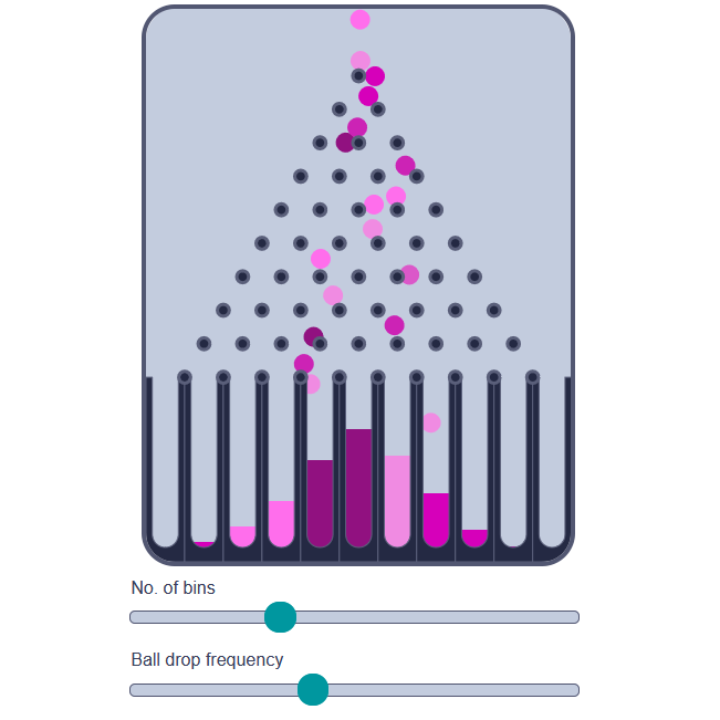
Bean machine
Virtual bean machine illustrates how the binomial distribution arises. Change the number of bins to see how the binomial distribution approaches the normal distribution as this number goes to infinity
Transformations
Flip switches to reveal graphs of the addition, multiplication, and exponentiation functions and drag values in coloured circles to change the output these functions produce
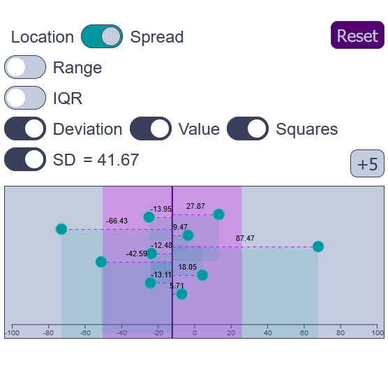
Descriptive statistics
Explore the various measures of central tendency and spread by adding and deleting points or dragging them around. You can select multiple points by dragging a rectangle across the plot
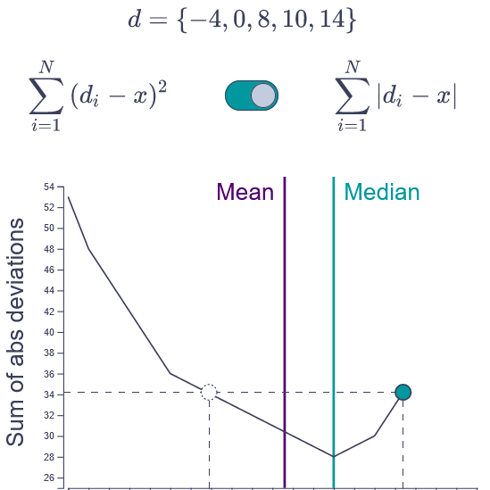
Squared vs absolute deviation
Compare the sum of squared deviations to the sum of absolute deviations of data from any point along the x-axis to find out why we use the former with the mean and the latter with the median
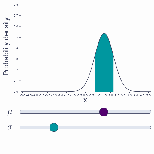
Normal distribution
Explore the two parameters that define the normal distribution – μ and σ – to see how they determine the shape of the location and spread of the bell curve
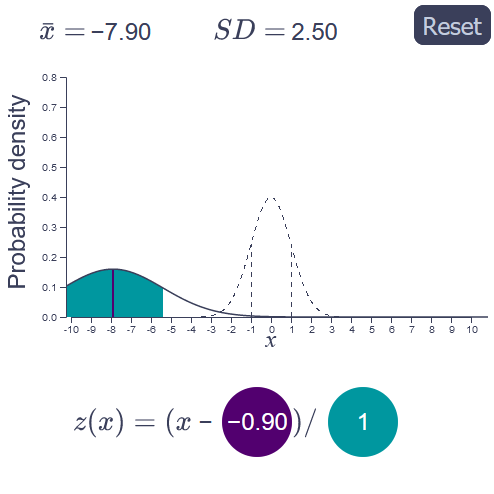
z-transformation
Change the centre and the scale of a randomly generated normal distribution to turn it into a standard normal distribution with μ = 0 and σ = 1. Watch out for order of operations though!
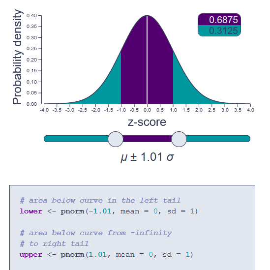
Area under the curve
Pick cut-off points along the x-axis and get the area below the standard normal curve within and outside of the range.R code to calculate area and cut-offs included!
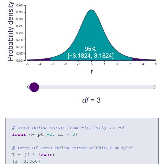
Student's t distribution
Change the number of degrees of freedom to see how the shape of the Student’s t distribution changes and how this change affects cut-off points for the outer 5% of the area under the curve
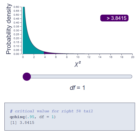
χ2 distribution
The shape of the χ2 distribution changes even more dramatically than the t distribution as the number of degrees of freedom increases
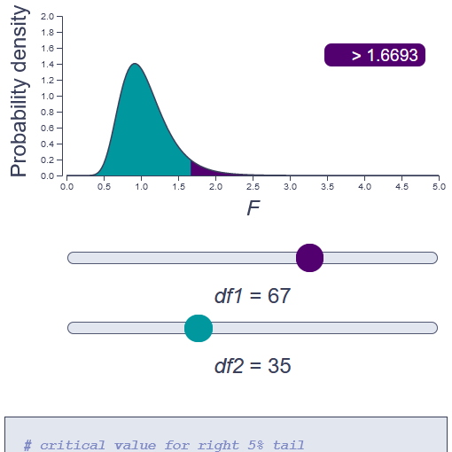
Snedecor's F distribution
The F distribution describes a ratio of two χ2 distributed variables (scaled by their respective dfs). See how the two degrees of freedom parameters determine its shape
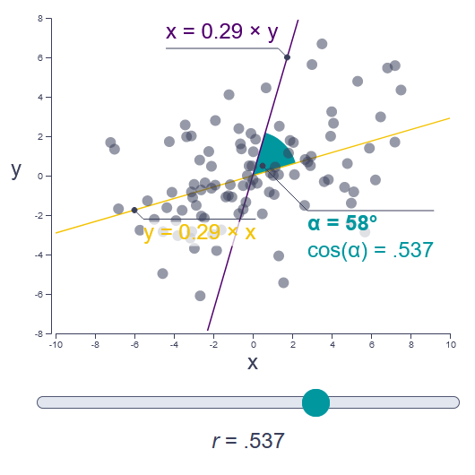
Correlation coefficient r
Discover the geometric representation of the correlation coefficient r to see that it is just the cosine of the angle between two lines of best fit drawn through the data
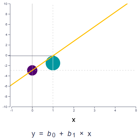
Linear equation
Play around with the intercept and the slope of a line to see how different values of the parameters of the linear equation determine the vertical position and the steepness of the line
Line of best fit
Ordinary Least Squares regression is one way to find the line of best fit through a scatter of data. Change the intercept and the slope to find this line
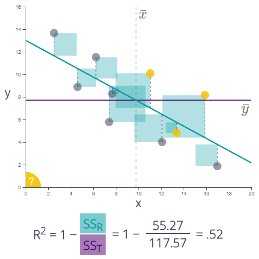
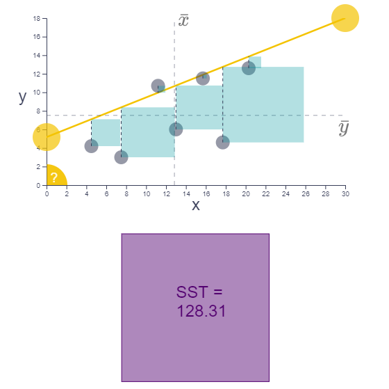
R2
R2 expresses how well the model describes the relationships in the data. Add and delete points or move them around to see how they influence both the line and R2