Looking Ahead (and Behind)

• Last week: Correlation

• This week: Chi-Square ( ${\chi }^2$ )

• Week 6: t-test

• Week 7: The Linear Model

• Week 8: The Linear Model

Lab Report: Green Study

• Today we will talk about one of the analyses for the lab report

  • ${\chi }^2$ : Green study (Griskevicious et al., 2010)

  • t-test: Red study (Elliott et al., 2020), next week

• We will talk about the lab report in the lectures and work on it in the practicals

  • Make sure you come to your registered sessions

Objectives

After this lecture you will understand:

• The concepts behind tests of goodness-of-fit and association

• How to calculate the ${\chi }^2$ statistic

• How to read tables and figures of counts

• How to interpret and report significance tests of ${\chi }^2$

• The relationship between association and causation

Roll of the Dice

Roll of the Dice

• I want to know if my four-sided die (d4) is fair

• If it is, each number should come up with equal probability

  • Four numbers = 100%/4 = 25% probability of rolling each number

• So, if I roll the dice 100 times, each number should come up (approximately) 25 times

Roll of the Dic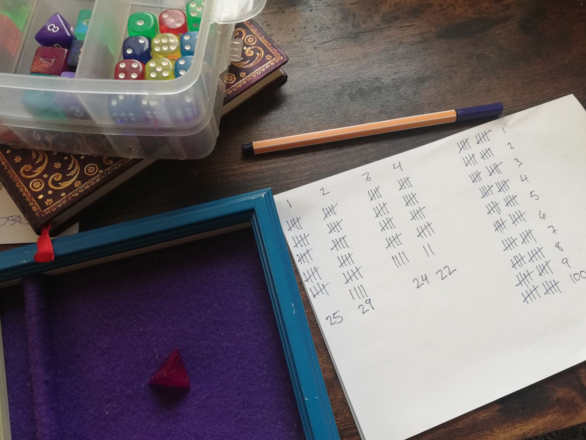e

A Fair Shake?

• These numbers are not exactly 25/25/25/25

  • But we live in a random universe!

• How different is different enough to believe that the die is not actually fair?

Steps of the Analysis

• Calculate the (standardised) difference between observed and expected frequencies

• Compare that test statistic to its distribution under the null hypothesis

• Obtain the probability p of encountering a test statistic of the size we have, or larger, if the null hypothesis is true

• ?????

• Profit

Step 1: Calculate a Test Statistic

• How different are the observed counts from the expected counts?

Step 2: Compare to the Distribution

• We've calculated a test statistic that represents the thing we are trying to test

  • Is this test statistic big or small in the grand scheme of things?

• Compare our test statistic to the distribution of similar statistics

  • IMPORTANT: These distributions assume that the null hypothesis is true!

The Chi-Square (χ²) Distribution

• Unfortunately test statistics like the one we have are not normally distributed

• No problem - we just have to use a different distribution!

• Meet the ${\chi }^2$ distribution

  • The sum of squared normal distributions

  • See this excellent Khan Academy explainer for more!

Detour: Degrees of Freedom

• Degrees of freedom are calculated differently for different test statistics

  • Important because they determine the distribution's shape and proportions

• At base, they are the number of values that are free to vary

• Consider our dice example...

  • We know our test statistic is 1.04

  • If we know the first three values (0 + 0.64 + 0.04), the last value must be 0.36

  • Alternatively, if we had three random values (e.g. 0.23 + 0.54 + 0.1), the last value cannot be random: it must be 0.17 to add up to 1.04

  • So, we have three degrees of freedom

Step 3: Obtain the Probability p

• Look at the distribution for 3 degrees of freedom

• What percentage of the distribution is greater than or equal to 1.04?

Interpreting the Results

• The sum of squared differences between our expected and observed counts ( ${\chi }^2$ ) was 1.04

• For a ${\chi }^2$ distribution with 3 degrees of freedom, this value is extremely common under the null hypothesis!

  • If our die is fair, our data are extremely likely

  • To believe that the die was not fair, we would have needed a test statistic of ~7.8 or greater ( $\alpha$ = .05)

• If only there were an easier way to do this...!

chisq.test(dice_table$obs_count)

## 
##     Chi-squared test for given probabilities
## 
## data:  dice_table$obs_count
## X-squared = 1.04, df = 3, p-value = 0.7916

Interim Summary

• The ${\chi }^2$ test statistic quantifies how different a set of observed frequencies are from expected frequencies

• We obtain the probability p of finding the test statistic we have calculated (or one even larger) using the distribution of the ${\chi }^2$ statistic under the null hypothesis, with a given number of degrees of freedom

• Given an $\alpha$ level of .05...

  • If p > .05, we conclude that our results are likely to occur under the null hypothesis, so we have no evidence that the null hypothesis is not true

  • If p < .05, we conclude that our results are sufficiently unlikely to occur that it may in fact be the case that the null hypothesis is not true

More χ²

• We just saw a goodness of fit test

  • Tests whether a sample of data came from a population with a specific distribution

• Next, let's look at a test of association, or independence

  • Are two categorical variables associated or not?

• For your lab reports, you will again write about the Green or Red studies

  • You can freely choose which!

  • If you choose the Green study, this is the test you will use

Quick Refresher: Variable Types

• Continuous data

  • Represent some measurement or score on a scale

  • Examples: ratings of romantic attraction, age in years

  • Answers the question: how much?

• Categorical data

  • Represent membership in a particular group or condition

  • Examples: control vs experimental group, year of uni

  • Answers the question: which one?

χ² Test of Association

• This time we will have two variables, both categorical

• Data: counts of how many observations fall into each combination of categories

Sequence-Space Synaesthesia

• Spatial orientation of sequences, such as numbers, months, or days of the week

Sequence-Space Synaesthesia

• "Calendars" of spatial orientations of months of the year

• Brang et al. (2011): Is the orientation of the calendar related to the synaesthete's handedness?

  • Orientation: months progress clockwise or counterclockwise in space

  • Handedness: left or right handed

Let's Think About This...

• What is the null hypothesis in this case?

• What is the alternative hypothesis?

• What do you think we will find?

Let's Think About This...

• Null hypothesis: Calendar orientation is not associated with synaesthete handedness

• Alternative hypothesis: Calendar orientation is associated with synaesthete handedness

• Prediction from the paper:

  • Right-handed synaesthetes will tend to have a clockwise calendar

  • Left-handed synaesthetes will tend to have an anticlockwise calendar

Visualising the Data

ggplot(ss_tab, aes(x = handedness, y = n)) +
  geom_bar(
    aes(fill = orientation), 
    stat="identity", position = position_dodge(0.8),
    width = 0.7) +
  labs(x = "Handedness", y = "Frequency", fill = "Calendar\nOrientation") +
  scale_y_continuous(limits = c(0, 20)) +
  scale_color_manual(values = c("#009FA7", "#52006F"))+
  scale_fill_manual(values = c("#009FA7", "#52006F"), labels = c("Anticlockwise", "Clockwise"))+
  scale_x_discrete(labels = c("Left","Right"))

• Left-handed synaesthetes have more anti-clockwise than clockwise

• Right-handed synaesthetes have the reverse

Test Result

Are these data different enough from the expected frequencies to believe that there may be an association between orientation and handedness?

## 
##     Pearson's Chi-squared test with Yates' continuity correction
## 
## data:  seq_space$orientation and seq_space$handedness
## X-squared = 9.7798, df = 1, p-value = 0.001764

Test Result

Are these data different enough from the expected frequencies to believe that there may be an association between orientation and handedness?

## 
##     Pearson's Chi-squared test with Yates' continuity correction
## 
## data:  seq_space$orientation and seq_space$handedness
## X-squared = 9.7798, df = 1, p-value = 0.001764

Interpreting the Result

ggplot(ss_tab, aes(x = handedness, y = n)) +
  geom_bar(
    aes(fill = orientation), 
    stat="identity", position = position_dodge(0.8),
    width = 0.7) +
  labs(x = "Handedness", y = "Frequency", fill = "Calendar\nOrientation") +
  scale_y_continuous(limits = c(0, 20)) +
  scale_color_manual(values = c("#009FA7", "#52006F"))+
  scale_fill_manual(values = c("#009FA7", "#52006F"), labels = c("Anticlockwise", "Clockwise"))+
  scale_x_discrete(labels = c("Left","Right"))

• Our hypothesis is supported by the data

  • The association is in the direction we predicted

Expected Frequencies

• Are these data different enough from the expected frequencies to believe that there may be an association between orientation and handedness?

  • We can get these easily out of R!

• One of the assumptions of ${\chi }^2$ is that all expected frequencies are greater than 5

  • Otherwise this test can give you a drastically wrong answer 😱

  • In this case, use Fisher's exact test (fisher.test()) instead

Final Overview

• The ${\chi }^2$ test quantifies the difference between observed and expected frequencies

• Goodness of Fit

  • Tests whether a sample of data came from a population with a specific distribution 🎲

• Test of Association/Independence

  • Tests whether two categorical variables are associated with each other 🌈

• Like with correlation, association is not causation

• For quizzes/exam:

  • You will not be expected to calculate ${\chi }^2$ by hand!

  • You will be expected to read and interpret the output of chisq.test() for tests of association

  • More in the tutorial!

Lab Reports

• You can choose either the red or green study to write your report on

  • See Lab Report Information on Canvas for more

• If you choose the green study (Griskevicius et al., 2010), you must use and report the results of ${\chi }^2$

• Choose one of three products to analyse

• Report observed frequencies and ${\chi }^2$ result

  • Include a figure of the results

  • Will be covered in depth in the next tutorial and practical!