In this lecture we will build on the understanding of the sampling distribution of the mean and the standard error developed in the previous lecture and talk more about the uncertainty that is inherent in estimation. We will learn how interval estimates can be used to quantify this uncertainty around point estimates. In particular, we will focus on the confidence interval and talk about how it is constructed using the t distribution and how to interpret it.
Objectives
The aim of this lecture is to help you understand
- the difference between point estimates and interval estimates
- what confidence intervals are, what coverage means, how they are constructed using the sampling distribution
- how the t distribution can be used to approximate the sampling distribution in situations when the standard error is not known and has to be estimated from the sample
- how to interpret confidence intervals
Before we dive in, let’s just reiterate what the point of doing statistics is. The reason why we are performing statistical tests and build statistical models of the world is to help us analyse and interpret the results of quantitative research. This research aims to describe and explain aspects of the world around us and make predictions about it. In statistical terms, the specific part of the world that a research study is focusing on can be viewed as a population and the particular aspect of interest can be seen as some parameter of this population. It can be anything really, the typical value in the population, the variability in the population, or the relationship between two or multiple variables in the population.
However, accessing and measuring the entire population and, by extension, observing these parameters is not possible for reasons we talked about on multiple occasions. The best we can then do is sample observations from the population of interest and estimate the values of these parameters based on some statistics calculated on the sample.
In other words, statistics is all about making inferences about populations based on samples. If we could measure the entire population, we wouldn’t really need statistics!
Point estimates
You’ve already heard of things like the sample mean, median, or mode. These measures of central tendency tell us about the “most typical” value in the distribution. Just like with everything, we don’t know the value of these measures in the population and when we calculate their values based on a sample for the purpose of doing statistics, we do so in order to get an estimate of what the value of the population parameter is most likely to be.
Estimates are essentially best guesses about the value of population parameters that we can make given the sample we have.
Because each one of these estimates is a single value representing some point along the range of the values of a variable, we call these estimates point estimates. Essentially, all estimates that are expressed as a single number are point estimates that represent our best guesses about the corresponding population parameters.
It’s not just the measures of location, however: Measures of spread (SD, \(\sigma^2\), etc.) are also point estimates, as they give us a single number that represents our estimate of the variability in the population.
There exist point estimates even for things like relationships between variables. The correlation coefficient r takes values from −1 to 1, where 0 is no relationship, 1 is a perfect positive relationship and −1 is a perfect negative relationship (see Figure 1).
df <- tibble(x = rnorm(100), y1 = rnorm(100), y2 = x + rnorm(100))
# values of r nicely formatted
r1 <- signs::signs(cor(df$x, df$y1), trim_leading_zeros = T, accuracy=.001)
r2 <- signs::signs(cor(df$x, df$y2), trim_leading_zeros = T, accuracy=.001)
# plots
p1 <- df %>% ggplot(aes(x, y1)) + geom_point(color = theme_col)
p2 <- df %>% ggplot(aes(x, y2)) + geom_point(color = theme_col)
# arrange plots and add nice titles
cowplot::plot_grid(p1 + ggtitle(paste0("*r* = ", r1)),
                   p2 + ggtitle(paste0("*r* = ", r2)))

Figure 1: Relationships between variables as single numbers: Left-hand-side plot shows no relationship (r almost 0) and right-hand-side plot shows a strong positive relationship between variables plotted on the two axes.
Accuracy and uncertainty
So to reiterate, a point estimate, such as the sample mean (\(\bar{x}\)) is the best estimate (\(\hat{\mu}\)) of population parameter, in this case \(\mu\). However, as we saw in lecture 1, the mean of almost any sample will differ from the mean of the population that the sample is drawn from. The same is true for any point estimate!
This is where the standard error (SE) enters the game. The SE of a parameter expresses the uncertainty about the estimate of that population parameter. Although we’ve only been talking about the standard error of the mean (SEM), it can be calculated for all point estimates, not just the mean.
Because SE gives us a kind of margin of error, we can use it to quantify uncertainty around point estimates and calculate so-called interval estimates.
Interval estimates
In addition to estimating a single value (i.e., a point estimate), we can use SE to estimate an interval around it. For instance, we can estimate \(\hat{\mu}\) based on our sample as having the value of 4.13 with an interval from, say, −0.2 to 8.46. Thus, by putting a range on the value of a point estimate, we communicate the uncertainty around it. The wider the interval, the more uncertainty we acknowledge with respect to our estimate.
There are different kinds of interval estimates appropriate for different scenarios, situations, and statistical methods. One of them, the confidence interval, is going to be of special interest to us.
Confidence interval
We can use SE – the standard deviation of the sampling distribution – to calculate a confidence interval (CI) with a certain coverage, e.g., 90%, 95%, 99%, around our point estimate. Let’s unpack what coverage is using an example.
Imagine we bought a bag of Minstrels with 200 chocolates inside. We can use the mean weight of a single Minstrel in sample of N = 200 to estimate \(\mu\), the population mean weight of a Minstrel.
First of all, we weight up the bag and record the weight in grammes. Then we divide the number by 200 to get the sample mean weight, let’s say \(\bar{x}\) = 4.11g. This is our best guess about the value of the population mean, our point estimate \(\hat{\mu}\)
Let’s now, for the sake of the example, assume that we know the parameters of the population of Minstrel weight: \(\mu\) = 4, \(\sigma\) = 0.56.
Check your understanding
You’re advised not to move on without correctly answering these questions first.
Question 1
With respect to the values above, what is the standard error of the mean weight of a Minstrel for N = 200?
Give answer to 2 decimal places.
0.04
Correct!That’s not right…
Question 2
What are the critical values (in terms of z-scores; scores from the standard normal distribution) that cut off the outer 5% of the distribution, leaving the bulk 95% of the area below its curve?
Give answer as a single number rounded to 2 decimal places, so 3.24 for a range between −3.24 and 3.24.
1.96
Correct!That’s not right…
We can apply the ±1.96 × SE range around our \(\hat{\mu}\) to get a confidence interval with a 95% coverage:
\[\begin{aligned}95\%\text{CI} &= \bar{x}\pm1.96\times SE\\&= \bar{x}\pm1.96\times 0.04\\&=4.11 \pm 0.0784\\&=[4.0316, 4.1884]\end{aligned}\] OK so we have our confidence interval with a 95% coverage (95% CI) but what does a 95% coverage actually mean?
For a 95% CI, 95% of these intervals around sample estimates will contain the value of the population parameter.
This means that if we got a hundred bags of Minstrels (with 200 pieces in each bag), calculated the mean weight of each one and constructed a 95% CI around each sample mean, we would expect 95 of these 100 confidence intervals to include the true value of the population mean, \(\mu\) = 4.
Now, as it happens, in our particular example, the interval does not include 4. It’s one of the 5% that “got it wrong”. Aren’t we lucky!
Let’s illustrate coverage using another example.
This time, we’re sampling bags of oranges, with 30 oranges in each bag. In the picture below, the cluster of circles represents the population of oranges. As you can see, they have different sizes. Again, we’re assuming that we know the true mean size of an orange, \(\mu\) = 10.7, as shown by the vertical red line in the right-hand-side panel.
Let’s sample our first bag of 30 oranges. Click/tap the picture once.
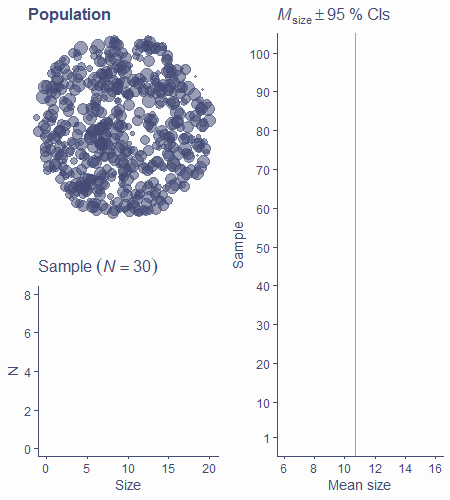
OK, the highlighted circles are our sampled oranges. Their sizes are plotted on a histogram below. Click/tap again…
Now, the mean size in the sample – our \(\hat{\mu}\) – along with a 95% CI is shown on the right-hand-side panel. You can see that the interval intersects the vertical red line. That means that this particular 95% CI around our estimate does indeed include the value of the population parameter.
Click again to start a resampling animation that will go on until we have 100 estimates with 100 CIs.
Right, so as you can see 5/100 CIs did not include \(\mu\) (did not intersect the vertical red line). So, in this case, our simulation is perfectly in line with the definition of coverage: 95% of the confidence intervals include the population mean, while the remaining 5% do not!
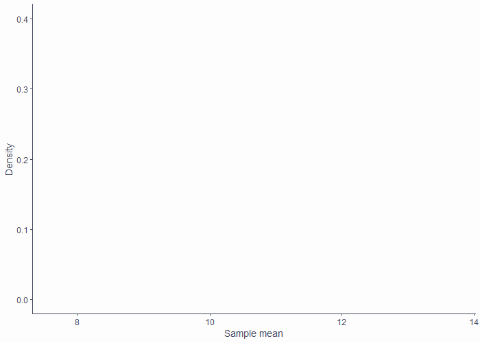
The animation below illustrates how a 95% confidence interval is constructed. If you were following the explanation above, this should make sense.
Putting the CI around our sample estimate is actually very easy if we know the exact specification of the sampling distribution. Click on the picture to draw the sampling distribution.
The green area represents the inner 95% of the sampling distribution. Because this distribution is normal (as per CLT), the borders of the green area lie at ±1.96 SE from the centre of the distribution. Click on the picture again to visualise this relationship.
We can use exactly this distance on each side of any given sample mean to construct the 95% CI. Just a few more clicks see this.
So there you have it, easy if we know the exact specification of the sampling distribution. But you can probably tell by the repeated emphasis that there’s a catch…
In this case, the catch is that the sampling distribution is never known. We will never know its mean (true population mean), nor will we ever know its SD (SE), which we need to calculate the range of the interval. The reason why we don’t know SE is that it is calculated using population standard deviation \(\sigma\), which, like any population parameter, we cannot measure.
And because of this, we have to approximate the sampling distribution using the t distribution. Before we can move on to discussing how this approximation is done, we need to talk about the t distribution a little.
The t distribution
The t distribution is more a family of distributions, because there are many different shapes. Just like the standard normal distribution, all of these shapes are symmetrical and centred around 0.
Unlike the normal distribution, however, the shape of any given t distribution changes based on a parameter called degrees of freedom.
With 1 degree of freedom (df), the distribution is very “fat-tailed”, meaning that a large proportion of the are under its curve lies in the tails, compared to the normal distribution. This shape gets more and more “normal-like” as the number of dfs increases and, when df = \(\infty\), the t distribution is identical to the standard normal distribution.
Have a little play around with this app to get a feel for the t distribution. Use the slider to change the df parameter that determines the shape of the distribution.
As you can see, when the shape changes, the proportions of the distribution change too.
Unlike in the standard normal, where the middle 95% of data always lie within ±1.96, this critical value in the t distribution changes based on df.
The t distribution crops up in many situations in statistics but when it does it always has to do with estimating the sampling distribution of a parameter from a finite sample.
Now you might be wondering how we calculate the number of dfs or what even are they. Well, as for the first issue, this changes based on context but often it has to do with sample size, N, number of estimated parameters, or both. In the case of approximating the sampling distribution of the mean, we calculate this number as df = N − 1.
And as for what dfs are, you can check out the “Extra” box below but you are not required to know this.
Degrees of freedom
As we said before, the concept of degrees of freedom is a little esoteric. Technically, it is the number of values that are free to vary in a system, given some constraints. (Told you so!)
Let’s talk about what this means on the example of a sudoku puzzle. The sudoku grid is our system, and the rules are our constraints (some requirement that we put in place).

The rules of the puzzle are
- Each row must contain all numbers between 1 and 9
- Each column must contain all numbers between 1 and 9
- Each one of the nine 3×3 boxes must contain all numbers between 1 and 9
Given these rules, there are A LOT1 of ways we can fill in an empty sudoku grid. The puzzle always provides several pre-filled numbers and the task is to complete the grid according to the rules. Here is an example of an unsolved and solved sudoku puzzle.

Now, When the board is empty, any individual field can contain any allowed number. In other words, its value is free to vary. But as soon as we fill in one field with, let’s say a 9, the rest of the fields in the same row, column, and box can only take values between 1 and 8. There are still many many solutions but fewer than before we entered the 9. Actual sudoku puzzles are set up in such a way that they only have one possible solution.
With that, let’s look at the definition again:
“Degrees of freedom is the number of values that are free to vary in a system, given some constraints”
So the degrees of freedom of sudoku is the minimum number of values we can enter into the grid so that there is only one possible solution to the puzzle. As it happens, there are 17 degrees of freedom in a sudoku. Giving any more than 17 clues just makes the one solution easier to find but, theoretically, you only need 17. It’s going to be some fiendishly difficult sudoku, mind you!
You might be wondering how this concept translates to the context of statistics and confidence intervals. Well, we said that the number of df for the t-distribution we use to get the cut-off value for the 95% CIs is equal to N−1. This is because we already constrained the value of the mean. So, if our bag of Minstrels has 200 chocolates in it and the mean weight of a chocolate is 4.11g, 199 of them can theoretically weigh any amount (if we allow negative weights) but, in order for the mean to be 4.11g, the weight of the last Minstrel is determined by the weights of the others.
And that’s why in a bag of 200 Minstrels, there are 199 degrees of freedom: df = N−1.
OK, now that we know some basics about the t distribution, let’s go back to CIs.
We said that 95% CI around estimated population mean is mean ±1.96 SE. This is absolutely true, but the problem is that we don’t know the value of SE because it’s calculated from population standard deviation \(\sigma\), which is also unknown. What we do instead is calculate the estimate of SE, \(\widehat{SE}\), from the sample standard deviation s.
Because of this one detail, we cannot use the normal distribution and its ±1.96 critical value. Rather, we approximate the shape of the sampling distribution using the t distribution. And because the shape of the t distribution changes as a function of df (and therefore sample size), the critical values for cutting off the outer 5% of the area change too. As a result, we need to replace the 1.96 with the appropriate critical value for the t distribution with a given number of dfs.
In our example with oranges, for our bag of N = 30, the critical value is tcrit(df=29) = ±2.045.
Of course, we can ask R to calculate the critical value for us:
qt(p = 0.975, df = 29)
[1] 2.04523So, a 95% CI around the mean for a sample of 30 is \(\bar{x}\) ±2.05 × \(\widehat{SE}\).
If you would like to know the full explanation for why we need to approxiamte the sampling distribution via the t distribution, check out the “Extra” box below.
To reiterate, here’s the full calculation for our bag of 200 minstrels with mean = 4.11 and s = 0.54:
First, the estimate of SE is
\[\begin{aligned}\widehat{SE}&=\frac{s}{\sqrt{N}}\\&=\frac{0.54}{\sqrt{200}}\\&\approx0.038\end{aligned}\] Now, what we have our estimate of SE (ass opposed to the true SE of 0.04), let’s plug it in along with our sample mean and the correct critical value of t to get the 95% CI:
\[\begin{aligned}95\%\ CI &= \bar{x}\pm t(N-1)_{crit}\times \widehat{SE}\\&=4.11\pm1.972\times0.038\\&=4.11\pm0.075\\&=[4.035, 4.185]\end{aligned}\]
Remember
To construct a 95% CI around our estimated mean, all we need is
- Estimated mean (i.e. sample mean, because \(\hat{\mu}=\bar{x}\))
- Sample SD (s)
- N
- Critical value for a t distribution with N − 1 df
Check your understanding
Let’s calculate one more 95% CI. In this example, we’ve bought another bag of Minstrels, this time with 100 chocolates in it. In this bag, the mean weight of a Minstrel was 4.02 with a SD of 0.62.
Given these statistics, answer the following questions.
Question 3
What is the estimate of standard error (\(\widehat{SE}\)) given our sample?
Give answer to 3 decimal places.
0.062
Correct!That’s not right…
Question 4
What is the critical t-value we need for calculating a 95% CI?
Give answer as a single number rounded to 3 decimal places, so 3.245 for a range between −3.245 and 3.245.
1.984
Correct!That’s not right…
Question 5
Finally, what is the 95% CI around our sample mean?
Give answer as a range of numbers rounded to 3 decimal place, for example 2.245-4.425.
3.897-4.143
Correct!That’s not right…
Why approximate via the t distribution?
The reason why using sample SD (s) instead of population SD (σ) for calculating the standard error forces us to use the t distribution has to do with the fact that the latter is a constant, while the former is a variable. Let’s elaborate.
There is only one population and so there is only one σ. However, there are almost infinite possible samples and each one has its own s. This matters because we are using SE to determine the width of the confidence intervals. This SE is based on a given s in our sample which might be different from s in another sample. Look at the formula for 95% CI that we used:
\[\begin{aligned}95\%\text{CI} &= \bar{x}\pm1.96\times \widehat{SE}\\&= \bar{x}\pm1.96\times \frac{s}{\sqrt{N}},\end{aligned}\]
where \(\bar{x}\) is the sample mean and N is the sample size.
In our Minstrel example, we said that we can use the ±1.96×SE range to construct a 95% confidence interval around the mean weight of a single chocolate we calculated from our bag of 200. Getting the s in the bag (0.54) and substituting in the formula, we get:
\[\begin{aligned}95\%\text{CI} &= \bar{x}\pm1.96\times \widehat{SE}\\ &= 4.11\pm1.96\times \frac{0.54}{\sqrt{200}}\end{aligned}\]
Make sure you understand the above because here comes the actual reason:
The ±1.96 cut-off for the most extreme 5% of the distribution only applies to the standard normal distribution (a normal distribution with mean = 0 and SD = 1). If the distribution is not standard normal, this cut-off doesn’t give us the middle 95% / tail 5% of the distribution. So in order to be able to use the cut-off in the formula:
\[\bar{x}\pm1.96\times \widehat{SE},\]
\(\bar{x}/\widehat{SE}\ \) must follow the standard normal distribution.
Now, we know that \(\bar{x}\) is a variable (each bag has its own mean) that does indeed follow the normal distribution (see Fig. 2). We can standardise it – turn it into the standard normal – by subtracting from it the mean of the sampling distribution from the variable and dividing it by SE. This is, however, only true if SE is a constant! The actual SE really is a constant because there is only one sampling distribution of the mean for N=200 and so there’s only one SE. But there are as many estimates of SE as there are samples and thus \(\widehat{SE}\) is a variable. What’s worse, it is not a normally distributed variable: it follows a different distribution, the Chi-squared (χ2) distribution.
Like the t distribution, the χ2 distribution also changes shape as a function of degrees of freedom. This is what the distribution looks like for a range of different number of dfs:
So, instead of dividing our \(\bar{x}\) by a constant SE, we are dividing it by a χ2-distributed variable. And, as it happens, the t distribution is exactly what happens when you divide a normally distributed variable by a χ2-distributed variable!
Because the difference between the normal and the t distribution is largest when N is small, let’s illustrate this on the example of a tiny bag of 5 Minstrels. If we divide \(\bar{x}\) by SE, we get a normal distribution (left branch of the plot below) and we can use the ±1.96 cut-off. That’s because 95% of a normal distribution lies within ±1.96 from its mean. However, in situations when SE is not known and is estimated as \(\widehat{SE}\), we are dividing by a variable and the resulting distribution is a t distribution with N−1 degrees of freedom (df) which had a different cut-off for 95% of its inner mass (±2.78 from the mean). This is the scenario in the right branch of the plot below.

This is the reason why we must use the t distribution in situations when we do not know the population standard deviation σ.
Interpreting confidence intervals
Ok so now that you know how CIs are made, let’s go over what they actually are once again. They are tricky beast them!
It’s important to remember that the width of the interval tells us about how much we can expect the mean of a different sample of the same size to vary from the one we got. Just compare the two Minstrel examples and you’ll see that each of the means lies within the confidence interval of the other.
Moreover, there’s a x % chance that any given x % CI contains the true population mean. In our first example, we got a little unlucky as our CI, despite having a 95% coverage, missed the population mean by a fraction. However, the other one did contain the value of \(\mu\).
Frustratingly, we can never know whether our particular CI does or doesn’t contain the value of \(\mu\). That’s just one of the uncertainties inherent in statistics. Don’t worry, you’ll get used to the discomfort it causes…
IMPORTANT CAVEAT
Saying that 95% of the CIs will contain the value of the true population parameter is not the same as saying that there’s a 95% chance that the population mean lies within our CI!
The kind of statistics we use treats population parameters as fixed: they are what they are, even though they are unknown. Because of that, we cannot talk about the probability of them being here or there.
Finally, remember that CIs can be calculated for any point estimate, not just the mean! Remember our Figure 1 with r coefficients representing the relationships between two variables? Well, we can put CIs around them too:
# Getting the plot titles right is rather involved
# and probably not worth the effort
r1 <- cor.test(df$x, df$y1)
r1_coef <- signs::signs(r1$estimate, trim_leading_zeros = T, accuracy=.001)
r1 <- paste0(
  r1_coef, "; 95% CI [",
  paste0(
    signs::signs(r1$conf.int, trim_leading_zeros = T, accuracy=.001),
    collapse = ", "),
  "]")
r2 <- cor.test(df$x, df$y2)
r2_coef <- signs::signs(r2$estimate, trim_leading_zeros = T, accuracy=.001)
r2 <- paste0(
  r2_coef, "; 95% CI [",
  paste0(
    signs::signs(r2$conf.int, trim_leading_zeros = T, accuracy=.001),
    collapse = ", "),
  "]")

# p1 and p2 are the same as before
cowplot::plot_grid(p1 + ggtitle(paste0("*r* = ", r1)),
                   p2 + ggtitle(paste0("*r* = ", r2)))

With this level of understanding of samples, populations, sampling distributions, standard error, and confidence intervals, you are now more than ready to learn about statistical testing.
But that’s a story for another day…
Take-home message
- Our aim is to estimate unknown population characteristics based on samples
- Point estimate is the best guess about a given population characteristic (parameter)
- Estimation is inherently uncertain
- We cannot say with 100% certainty that our estimate is truly equal to the population parameter
- Confidence intervals express this uncertainty
- The wider they are, the more uncertainty there is
- They have arbitrary coverage (often 50%, 90%, 95%, 99%)
- CIs are constructed using the sampling distribution
- True sampling distribution is unknown, we can approximate it using the t distribution with given degrees of freedom
- CIs can be constructed for any point estimate
- For a 95% CI, there is a 95% chance that any given CI contains the true population parameter
Apparently about 6.7×10²¹, according to this paper↩︎