Welcome to the first (well, zeroth) Analysing Data tutorial, where you’ll learn some cool and useful R Markdown tricks that will help you write better documents.
Objectives
- Consolidate what you’ve learnt about R Markdown last term
- Introduce basic code chunk options
- Discuss additional YAML arguments for customised documents
- Showcase a few Rmd tricks
- Take first steps towards writing papers/reports
Setup
Just you did in Psychology as a Science, before you start working on this week’s content, make sure to:
- If you haven’t done so yet, create a folder dedicated to all things related to this module. You can call it “02_and” or “02_analysing_data” and it should live in the same folder as your “paas” folder
- In RStudio, create a “week_01” R project (underscores instead of spaces and 01 instead of 1!)
- Once the project has been opened, create the standard folder structure inside:
- “data”
- “r_docs”
- “scripts”
- Download this accompanying Rmd file and save/move it in the “r_docs” folder. Make sure the file is saved as a .Rmd file and not as a .txt file!
- Open the file in RStudio and run the first code chunk labelled
setup.
Task difficulty
The tasks in this worksheet vary in difficulty and complexity. While you are absolutely capable of completing all of them, the harder ones may require you to get more practice before you can tackle them with confidence. Don’t be disheartened if you can’t figure them out straight away. Just come back to these tasks after a week or two, once the new knowledge has had some time to settle.
There are four difficulty levels in this worksheet. To make them a little more fun, they’re named after music genres. Sorted from easiest to hardest these are:
| Difficulty | Description |
|---|---|
| punk! | Easy, warm-up stuff. Just like the music genre, these tasks are not very complex. Unlike the songs in the genre, the tasks don’t need to be political to be good. |
| Prog-rocK | Medium difficulty – some creativity and thinking required. To quote a wise man: “I started listening to progressive rock in the early 70s and some of the songs have yet to end.” |
| jazz… | Jazz is hard and so are these tasks: technical, complex, at times confusing. They may require several attempts over a period of time so don’t give up! |
| death metal | These tasks would make even your teachers break a sweat so don’t worry if you can’t nail them. (Not that death metal is technically more difficult than jazz; it just can be VERY hard to listen to.) |
Want more?
If you’re keen to learn more about R than strictly necessary, you can find additional tips, tricks, and info in the gimme moR! boxes.
Rmd code chunks
Chunk labels
As you probably know by now, code chunks are just blocks of R code in your R Markdown file.
For R to recognise these as code and not as just any old text, they must be fenced off using:
```{r optional-label, [chunk options]}
[some R code]
```
The labels are completely arbitrary and it is up to you whether or not you use them.
The benefit of naming code chunks using labels is that, if your document fails to knit because there’s an error in one of your code chunks, R will tell you the label of the offending chunk.
Good examples of chunk labels are things like: data-processing, analysis, data-viz, desc-table, etc.
A minimal code chunk looks like this:
```{r}
[some R code]
```
Notice that there are no blank spaces before or after the three backticks and the r is lower-case.
This is important so make sure you conform to these rules.
The easiest way of inserting code chunks is either using the “Insert” menu at the top of your editor pane or using the Ctrl + Alt + I (Windows) or ⌘ Command + Option + I (MacOS) shortcut.
There are also some basic style rules for labelling code chunks:
- Keep them short
- Do not use spaces, use dashes “-” instead
- Do not start with a number
- Use only lower case letters
- Only use basic english alphabet letters and numbers
Chunk options
Chunk options are basically arguments to the function that formats the chunks when your document is knitted. You can use them to change the look of the chunk’s result.
To set a chunk option, add it to the opening fence:
```{r, option-name=value}
Notice the comma after r.
It must be there!
Different options are useful for different things so it is a good idea to have an understanding of what the options do. Let’s look at the three most commonly used
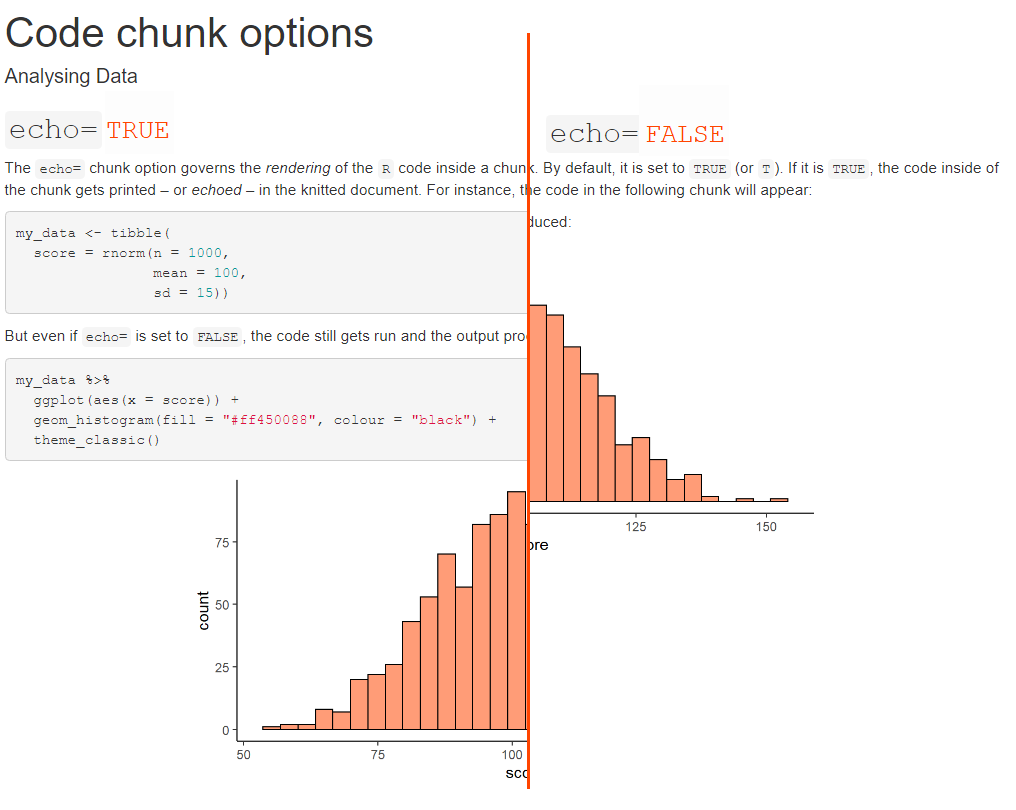
The echo= option
This option determines whether or not the code (not the output!) gets printed in the knitted document.
By default, it is set to TRUE for all chunks.
If you don’t want the code to be visible, just change the option to FALSE.
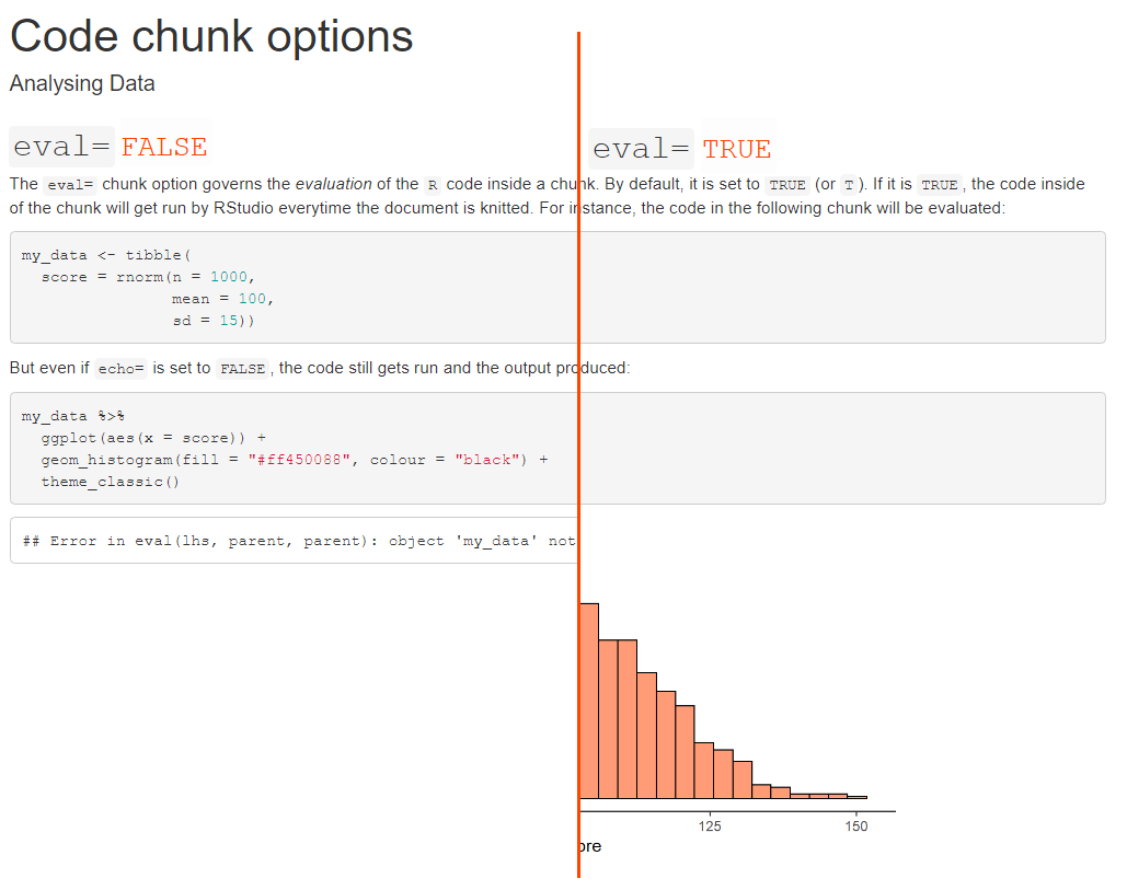
The eval=option
The eval= option decides whether or not R will run the code in the chunk.
If TRUE (default value), the code gets evaluated.
But if you change it to FALSE for a given chunk, none of the commands within that chunk will get executed.
In the picture below on the left side, the code used to create my_data does not get evaluated.
This has a knock-on effect on the subsequent chunk.
As there is no my_data, we get an error when trying to use this object to plot the histogram.
The include= option
This option determines whether both code and output appear in the knitted document.
It does not change evaluation, though: regardless of its value, the code gets executed by R.
But, if the option is set to FALSE this will happen quietly in the background and there will be no record of this happening in the knitted document.
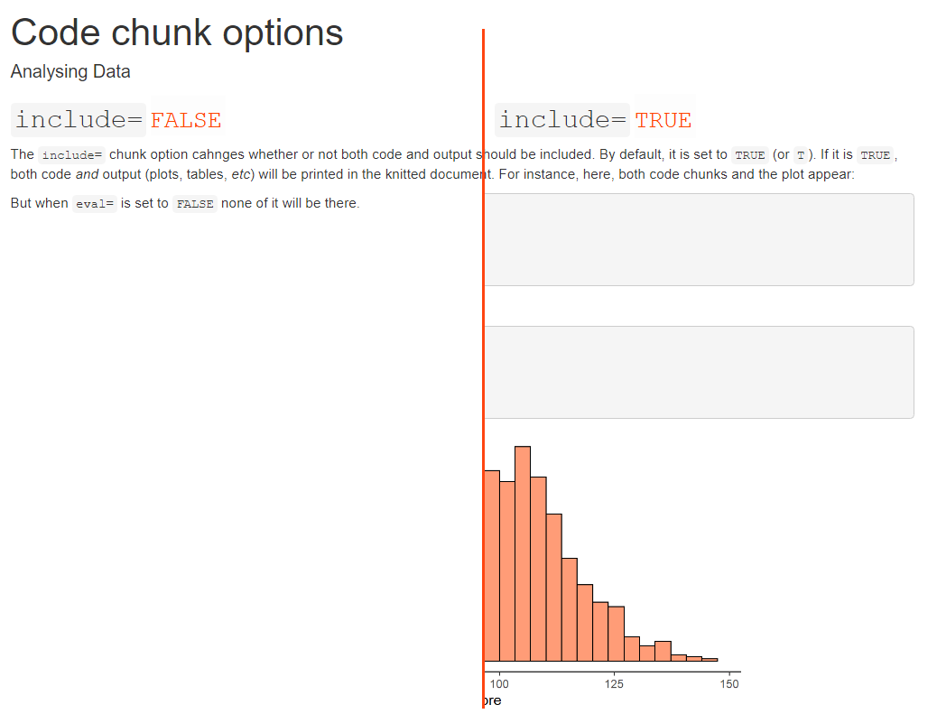
Notice that the setup chunk in a new Rmd file is set to include=FALSE.
That is why it never appears in the knitted document.
Usage
include=FALSE- For code whose output you never want to show
- e.g.,
library()calls, data processing and analysis code, or thesetupchunk
echo=FALSE- When you want output but not the code
- e.g., plots and tables
eval=FALSE;echo=TRUE- When you want to demonstrate code but don’t want to run it (rarely)
Setting options globally
You’ve probably already noticed that the setup chunk gets put into every new Rmd file.
We can edit it to set global options that will then apply to all subsequent chunks.
To do that. simply change/add the echo=, eval=, or include= options (or others) within the knitr::opts_chunk$set() function you’ll find in the chunk:
```{r setup, include = FALSE}
knitr::opts_chunk$set(echo = FALSE, include = FALSE)
```
Setting options locally
Any individual code chunk can be given its own options.
If you do this, it will override any global options that you might have set in the setup chunk.
For instance, even if echo= is set globally to FALSE, the following chunk gets echoed in the knitted document
```{r demo_chunk, echo=TRUE}
my_data <- tibble::tibble(
  score = rnorm(n = 1000,
                mean = 100,
                sd = 15))
```
Using the YAML header
You’ll recall that the YAML header is the bit at the very top of your .Rmd file, fenced off by a couple of ---s.
It is used to set title, subtitle, date, author name, format of the knitted document, and various bits meta-data.
Thus far, we have been using html_document in its default form as our output format.
Let’s have a look at how to change the look of our HTML document.
html_document: options
Output format can be modified using options set inside the YAML header.
When using HTML document, the html_document: bit must be on a new, indented line, followed by a colon :.
Any options we then want to set must be also on a new line and indented.
The whole thing looks like this:
---
title: "Code chunk options"
author: "Analysing Data"
output:
  html_document:
    option_1: some_value
    option_2: some_value
---
While R generally doesn’t care about line indentation, YAML – which is a different language – does and so it’s really important that the lines above are correctly offset.
Also notice below that, while in R we must spell TRUE and FALSE in all caps, in YAML, these must be lowwer case!
Let’s look at a few options now.
The toc: true option
We can enable a table of contents (toc) by setting the option to true.
Notice that YAML uses small letters for true, unlike R.
It also uses the colon to pass values to arguments, and not = like R does.
Finally, YAML really cares about the new lines and indentations, so pay attention to those things too!
---
title: "Code chunk options"
author: "Analysing Data"
output:
  html_document:
    toc: true
---
The resulting HTML document now has a table of contents right underneath the header. You can click on an individual heading to navigate to that particular section of the document. Handy, isn’t it?
The toc_float: true option
Setting toc_float to true puts the table of contents on the side of the file and keeps it there as we scroll down the document.
Try it below!
---
title: "Code chunk options"
author: "Analysing Data"
output:
  html_document:
    toc: true
    toc_float: true
---
If you cannot see the table of contents floating in the left margin, whe browser window is too narrow.
toc must be set to true in order for toc_float to take effect!
The number_sections: true option
Sometimes, we may want our section headings to be numbered. There’s an option for that too:
---
title: "Code chunk options"
author: "Analysing Data"
output:
  html_document:
    number_sections: true
---
See the result:
The reason why the headings are numbered 0.1 etc. is that, in this particular .Rmd, we didn’t use any level 1 (#) headings and started with level 2 headings (##). Only headings after and including the first level 1 heading are numbered 1. Anything before is the section 0.
The theme: option
Sometimes, you might want to customise the look of your document.
Since doing this requires knowledge of a completely different language (CSS), we will not be covering this.
However, there are several readymade themes you can choose from using the theme option:
---
title: "Code chunk options"
author: "Analysing Data"
output:
  html_document:
    theme: darkly
---
Using the darkly theme turns everything a little goth:
Take-home message
- Chunk options can change whether or not:
- Code chunks get echoed
- Code gets evaluated
- Code and output are included
- There are further options (see here)
- There are many YAML options to customise the formatting of the document, e.g.:
- Table of contents, including float
- Numbering of sections
- Themes
- Many other YAML options (see here)
That’s enough explaining. Now for some fun tasks!
Your turn
Task 1
If you haven’t done so yet, download the Rmd for this week’s tutorial (tut_00_rmd.Rmd) into the “r_docs” folder your “week_01” R project folder.
Task 2
Open this link and read the document.
This is a little tongue-in-cheek paper (well, by far not a complete paper) but, silly as it may be, it does have the proper structure of a piece of academic writing:
- Introduction
- Method
- Participants
- Materials
- Procedure
- Analysis
- Results
- Discussion
In the following weeks, we will learn how to write the Method, Results, and Discussion sections. We will be practicing exactly what you will need to submit for your lab report assessment so stay tuned!
Task 3
In the .Rmd, change the title to “Silly paper” and author to your name.
Just edit the first 2 lines of the YAML header to, for example:
---
title: "Silly paper"
author: "Russell Bell"
...[header truncated]...
---
Notice the special characters in Milan’s surname and how they appear in the .Rmd file.
These weird bunches of characters beginning with an ampersand, &1 and ending with a semi-colon, ; are so-called “HTML entities”.
Every letter or symbol that is not in the basic character set has an associated HTML entity.
For instance, the accent on á in Milan’s name is called an “acute” accent, which is why the HTML entity for an “a” with an acute accent is called á.
If you know what the character’s name is, you can easily look it up.
You can also find nice reference charts, such as this one.
HTML entities can only be used with HTML and Word output documents. If you want to knit into PDF, they will not work. Instead, you have to use a different kind of markup language called LaTeX /lay-tec or lah-tec/. Without going into details, here is a list of characters and their LaTeX codes
Task 4
Disable numbering of sections.
You can always check if anything you did worked by knitting the document (Ctrl + ⇧ Shift + K on Windows/Linux or ⌘ Command + ⇧ Shift + K on Mac OS).
You can either delete the number_sections: true line or just comment it out:
---
...[header truncated]...
    toc_float: true
    number_sections: true
    theme: spacelab
...[header truncated]...
---
Task 5
As you can see in the knitted file, there is a button to the upper right of every chunk that allows you to hide/show the code. Disable this option.
You might have to delete (or comment out) something from the YAML header…
Again, either delete the code_folding: show line or just comment it out. Changing the option to hide will result in the code being folded by default but still accessible with the buttons.
---
...[header truncated]...
    highlight: pygments
    # code_folding: show
    df_print: paged
---
Task 6
Look at the quote from The Raven and the footnote after the first sentence and notice how they are created in R Markdown. Chances are the knowledge will come in handy at some point.
Block quotes are formatted using a > followed by a blank space (see the .Rmd file)
To create a footnote, put [^1] immediately after the word where you want the number ot appear and then, in a paragraph of its own, put
[^1]: Your actual footnote.
Task 7
Set echo= to FALSE globally and knit the file to see the changes.
It’s done in the setup chunk.
Change the setup chunk to:
```{r setup, include = FALSE}
knitr::opts_chunk$set(echo = FALSE)
```
Task 8
The list of parts of the eye is misaligned. Make all items on the list the same level of indentation.
For the items to appear at the same level of the list, they must be all aligned in the .Rmd file
The organ has the following parts:

  - Cornea
  - Sclera
  - Pupil
  - Lens
  - Iris
  - Retina
  - Probably many more but what do we know!
Task 9
Something has gone wrong with the ## Materials section.
Look at the Rmd file and how the markdown got knitted in the document. The Materials subsection didn’t get created and the heading is still somewhere under participants. Can you fix this?
There is an empty line missing between the end of the “Participants” section and the “Materials” heading. You need to insert it:
## Participants

Data from `r nrow(my_data)` participants were collected (*M*~Age~ = `r my_data %>% pull(age) %>% mean(na.rm = T) %>% round(2)`, *SD*~Age~ = 1.46).

## Materials
Task 10
Table 1 is rounded to three digits. Change it to two digits.
Number of digits is an argument of the kable() function in the tab1 chunk. Just change it to 2:
```{r tab1}
...[code truncated]...
	# Tables should have captions
    caption = "Table 1. Descriptive statistics of the sample by eye colour",
    digits = 2) %>%
  kable_styling(full_width = FALSE) # for nicer formatting
```
Task 11
Make the plot bigger and knit the file to see all your changes.
You can manipulate the height and the width of the figure independently. Look at the corresponding code chunk.
Looking at the fig1 chunk, fig.height= and fig.width= are chunk options that set figure dimensions. You can experiment with different values and see what results they yield.
```{r fig1, fig.height=4, fig.width=5, fig.cap="*Fig.* 1  Age by eye colour. Error bars represent ±1 *SD*"}
my_data %>%
  group_by(eye_col) %>%
  summarise(n = n(),
  ...[code truncated]...
```
Very well done!
Today, you have revisited and expanded your knowledge of R Markdown. You learnt how to manipulate code chunk output and how to change default HTML document options in the YAML header. That is all for today, unless you’re a keen bean, in which case carry on to some more challenging but all the more rewarding tasks!
Extra tasks for the brave and keen
Task 1
Change your name to include special characters. If your name doesn’t have any, pick some for funsies – it’s metal time!
Just include HTML entities of the characters you want, for example:
---
title: "Silly paper"
author: "Ru$$ell Bell"
...[header truncated]...
---
Task 2
Looks at how date is specified in the YAML header.
As you can see, we can include R code in YAML, provided it’s in an inline code chunk (`r … `) and surrounded by quotes.
Task 2.1
Run the Sys.Date() command in your console to see what it does.
Task 2.2
Check out documentation for format() by typing ?format.POSIXct in the console and pressing Enter.
Scroll down until you come across a list of these weird %a, %A, … strings.
Read what the ones we used in the date YAML field and see how they translate into how the date is displayed in the knitted file.
Task 2.3
Get the date to appear in the DD/MM/YYYY format.
We need the %d for day number, %m for month number, and %Y (upper case) for full year. Don’t forget to include the slashes (/) and put everything in quotes!
To put this command into the YAML header, you need to write it as:
---
title: "Silly paper"
author: "Ru&apm;dollar;$ell Bell"
date: "`r format(Sys.Date(), '%d/%m/%Y')`"
...[header truncated]...
---
Notice that the entire command after date: is in double quotes and so the '%d/%m/%Y' string must be in single quotes.
Task 3
Comment out (Ctrl + ⇧ Shift + C on Windows/Linux or ⌘ Command + ⇧ Shift + C on Mac OS) the df_print line in the YAML header, knit the document and see what happens with the way the data set is printed towards the beginning of the file.
This YAML option changes the way data frames (and tibbles) are printed in the knitted file. Just see for yourself!
---
...[header truncated]...
    highlight: pygments
    code_folding: show
    # df_print: paged
---
Task 4
While the tabs under the Method section are pretty cool, they’re not really fit for a paper/report. Can you make the subsections appear as they usually do?
There is something unusual in the bit of the Rmd file where the Methods section gets created.
It’s this bit right here:
  - Probably many more but what do we know!


# Method {.tabset .tabset-pills}

## Participants
Delete it and see what the knitted document looks like.
Actual papers don’t use this tabbed layout and neither should your report!
Task 5
Edit the .Rmd file on line 87, so that the value of the standard deviation of age (SDAge) is knitted programmatically. By that we mean using code so that you don’t have to type in the value yourself.
Just like the other numbers in the sentence…
Data from `r nrow(my_data)` participants were collected (*M*~Age~ = `r my_data %>% pull(age) %>% mean(na.rm = T) %>% round(2)`, *SD*~Age~ = `r my_data %>% pull(age) %>% sd(na.rm = T) %>% round(2)`).Inline R code
This is known as in-line code: anything in the body text of a Rmd file surrounded by `r … ` will be interpreted as R code and evaluated before the document is knitted.
In-line code is a powerful tool that allows us to write technical reports (such as analysis reports) in a smart way without having to type in numbers manually.
We will talk more about in-line code next term but in principle, it’s the same as normal R code. However, because its output ends up pasted into the body text the code must only produce a sinle number or character string!
You are amazing!
Fun fact: the ampersand symbol “&” comes from a ligature of the latin word et [and]. In some fonts, the character still vaguely resembles Et.↩︎